Sandbox Survey

Introduction
     In the previous lab, we collect elevation points for a 114x114 cm sandbox. The data points were collected using a systematic sampling method collecting sample points every 6 cm within the grid. Once the elevation data was recorded it was then transfered into an excel spreadsheet. The data then needed to be normalized to decreased error and ease processing. Normalization refers to cleaning up data so that it uniform and easy to work with. Because a systematic sampling method was chosen for the initial survey, the data was already organized in evenly spaced increments. This allowed for the normalization to be very easily (figure 1).
     The objective for this lab was to take the topology data collected in the previous lab and create 3D topographic profiles in ArcMap and ArcScene. This was done using five interpolation methods 1) spline, 2) IDW, 3) natural neighbor, 4) kriging, and 5) Tin. Each of the methods produce different results when given the same data, because of this each of the interpolation methods will be explained in further detail below.

Figure. 1 Excel sheet displaying the normalized data collected in the previous lab

Methods
     Before the data could be interpolated into 3D topographic profiles, the data needed to be imported into ArcMap. To do this the add X,Y data tool was used create a new shapefile within a newly created feature class in a new geodatabase. The data for this project was left unprojected because the data was not collected using a geographic coordinate system, rather our own coordinate system (see lab 1 for details). Once this was completed the data could then be interpolated. After being interpolated, the models were brought into ArcScene where they were turned into 3D models.

• Spline: The first interpolation method was spline. Spline uses mathematical estimate values that reduce the curvature of a surface, passing through the center of the data points. This results a profile with a smooth surface. Spline is an effective method when there are a lot of data points but is not optimal if there are few data points as the model tends to over-correct, resulting in a overly simplified profile built upon generalizations. If there are large discrepancies in the elevation of data points that are close together, the model struggles to create realistic profiles. 
• (Inverse Distance Weighted (IDW): The IDW method estimates cell values by averaging the values of the collected data points using a weighted scale based upon relative distance to the sample point. For example, if a cell is closer to the sample point, it will have a higher weight assigned to that cell in comparison to a cell further away.
• Natural Neighbor: This method places a strong importance on the sample points themselves and creates regions surronding each point. 
• Kriging: This method is more complex than the previous methods as it uses formulas to create an estimated surface based upon sample point values. This model takes into consideration the correlations between direction and distance to predict a surface.  
• Triangulated Irregular Network (TIN): Tin models are created using set of vertices (sample points) to create a triangulated network using Delaunay triangulation. TIN models create high resolution areas where there is high amounts of variability between points and lower resolution models where data points have low variability. 

     Once the models were run, 2D topographic profiles were created, where they were later imported into ArcScene to create 3D topographic profiles.

Results
Spline: The first interpolation method was spline (figure 2). This created a smooth surface that accurately portrayed the surface of the sandbox. Areas in the southwest corner were over generalized as they were more flat in sandbox than the model portrayed. Of the five interpolation methods, this produced the most aesthetically pleasing model.

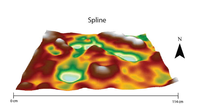Figure 2. Spline 3D interpolation model

IDW: The second model used was the IDW interpolation method (figure 3). This model does portray the elevation changes in the sand box quite well, however the model fails to smooth the surface. This produces a model that has unusual looking bumps that make the model appear unrealistic.

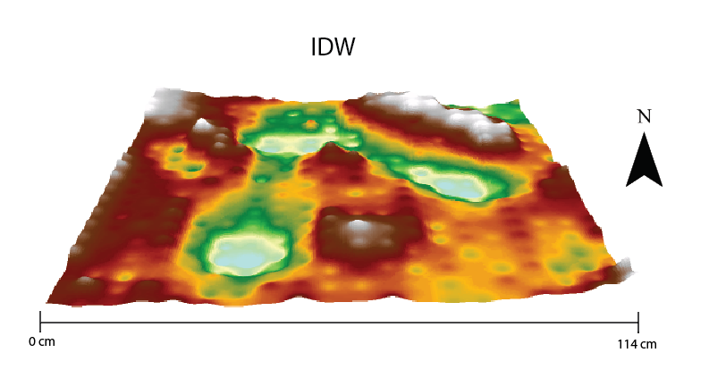Figure 3. IDW interpolation 3D model

Natural Neighbor: The next interpolation method used was natural neighbors (figure 4). This method produced a smooth surface that portrayed the surface accurately. Although the model is smooth, it lacks detail in areas of higher elevation changes than other models used.

Figure 4. Natural Neighbor 3D model

Kriging: The next model run was kriging (figure 5). This model gives a very basic profile of the sandbox. While the general surface of the model gives a general idea of what the topology of the sand box looked like, however the model leaves a lot to be desired in terms of detail.

Figure 5. Kriging 3D interpolation model

TIN: The final method used was TIN (figure 6). This method accurately portrayed the various elevations very accurately and provided an accurate representation of the sandbox. The model however doesn't portray the surface accurately as the triangulations give the model a more jagged look than the topology of the sandbox.

Figure 6. TIN  3D interpolation model

Summary
     Each of the methods used to create the 3D topographic profiles created unique models as each used different methods to achieve their final result. Of the five, the spline method created the most accurate representation of the sandbox. This was because of systematic sampling method combined with of samples relatively small area, allowed for the model to create a very accurate profile. Some of the other sampling methods would have been more appropriate had the study area been larger a more broad sampling method been applied. Interpolation models are not limited only to elevation models, but can be applied to precipitation, temperature, and even air pollution models.