Processing UAS Data

Introduction
This lab is an extension of our previous lab introduction to Pix4D, however in this lab we asked to process a set a unmaned aerial systems (UAS data. This data included ground control points (GCPs). GCPs improve the spatial accuracy of data by providing reference points for the data to be referenced to.

Methods
To begin the lab we were given a set of UAS data collected by Dr. Hupy (fig. 1). This data consisted of 69 separate UAS images. Before we began processing the data, we had to verify that the data was correct. Pix4D has integrated setting and perameters for different sensors and cameras. The software also reads the images metadata and then assigns the image a set of parameters. To begin we had to verify that the initial parameters were correct. We verified that the correct coordinate system was assigned to the data set. The data was given the WGS UTM Zone 15N coordinate system, which was correct. We also has had to change the camera type to a rolling shutter. We also set initial parameters for our data processing which involved only running the initial processing processing function. This was done to improve processing speed as we still had to make corrections to the GCPs. We also checked the google maps and kml boxes for the final product. This function allows for the data to be shared to a broader audience who may not have access to Pix4D pr ArcMap software. We also created shapefile for the data that consisted of contour lines which when brought into ArcMap would aid in mapping.

Figure 1. The image above displays the study area. The blue crosses seen within the image are the ground control points

Once the previous steps were completed, we were then asked to bring in GCPs. To do this we imported the CGPs using the Y,X,Z format. Once this was done we began the final processing of the data. Once the final processing was completed, we were given a quality report displaying the accuracy of the data (fig. 2). There was an error reported but this corrected later in lab when the GCP location was corrected (fig. 3).

Figure 2. First quality report generated after processing the data

Figure 3. GCP accuracy assessment 

The next step of lab was to correct the location of GCPs.  This was done manually insure that the GCPs were in an accurate location (fig. 4). 

Figure 4. Corrected GCP

Once the GCPs were calibrated (fig. 5), the data was then reoptimized. The Point Cloud and Mesh and DSM, Orthomosiac and Index were then checked on to finish the final processing. Once this was completed an orthomosiac and digital surface model (DSM) were created were they could later be brought into ArcMap. 

Figure 5. Data set in Ray Cloud once the GCP location was corrected

Results

After the data finished processing, it was brought into ArcMap to create a maps of the study area (fig. 6). The DSM and Orthomosiac images were displayed with hillshade, giving the images a 3D effect. The data did not show any errors in terms of the accuracy between the mosiaced image as there no distortions or gaps in the images. The DSM is pretty simple as the study area did not have a lot of variability in elevation. 

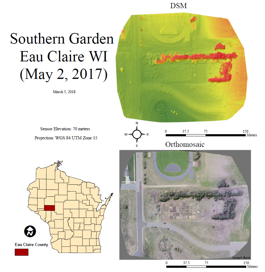Figure 6. The maps above display the Orthomosiaced and DSM images processed in Pix4D and displayed in ArcMap/

Conclusion

This lab showed that Pix4D is a useful software program for processing UAS data and converting the data into formats that are useful in other mapping softwares such as ArcMap and Google Earth. For the case of this lab, the UAS data set was quite small, but it provide valuable expiernce in processing UAS data as this a growing field within the geospatial community.